Running

Setup

If you are in a new shell, you need to setup SimpleAnalysis again. Follow the steps in the "On every login" part of the setup. If you have done the previous part of the tutorial already in your shell, you should be good to go without having to setup everything again.

Command line interface

Once setup, you will have the simpleAnalysis command available. Test this by entering simpleAnalysis --help into your shell. This should reveal the following set of options and arguments:

Run one or more truth-level analyses:
  -h [ --help ]               print usage and exit
  -o [ --output ] arg         Output name - if not supplied use analyses names
  -a [ --analyses ] arg       Comma-separated list of analyses to run
  -l [ --listanalyses ]       List available analyses and exit
  --input-files arg           Comma-separated list of input files
  -n [ --ntuple ]             Fill ntuple
  -M [ --multiRuns ] arg (=1) Run over each event multiple times - meant for
                              smearing analysis only
  -w [ --mcweight ] arg (=0)  MC weight index to apply (set to -1 to ignore it,
                              i.e. =1.)
  --nevents arg (=-1)         number of events to run on (set to -1 to ignore
                              it
  -T [ --useTrueTau ]         use true tau 4-vector instead of visible tau
                              4-vector
  --ignoreTruthBSM            ignore BSM truth blocks and use directly
                              TruthParticles (needs TRUTH1 input)
  -p [ --pdfReweight ] arg    PDF reweight to '<pdfName>[,energyIn,energyOut]'
  -P [ --pdfVariations ] arg  PDF reweight to '<generatedPdfName>'
  -D [ --decay ] arg          Decay HS particles '<pdgId=Lifetime in
                              ns>[,seed=number][,status=status-code]'

Running over a list of analyses and some inputfiles is as easy as running:

simpleAnalysis [-a listOfAnalysis] <inputFile1> [inputFile2]...

where listOfAnalysis is a comma-separated list of analysis (or all analyses if none are given). This will, for each analysis, provide acceptance results in a text file as well as a ROOT file containing all the histograms defined in the analysis routine.

Here is a short list of very useful command line arguments:

• Ntuple output

  If the -n option is provided, the output ROOT file will also contain an ntuple of all the variables defined in the analysis code.

• Output format when using multiple analyses

  By default, one pair of files (a text file and a ROOT file) is produced per analysis. If the option -o is provided, only one total pair of files is produced. In this case, everything inside these two files is prefixed by the analysis names in order to prevent naming clashes.

• MC event weight settings

  The option -w allows to change which event weight index is used to fill ntuple branches and histograms as well as compute the acceptances. You can disable event weights completely by setting this to -w -1.

If you have not already copied the inputs, please go ahead and do this now. The inputs section in the setup guide describes where and how to get the necessary inputs.

Local running

Let's run the analysis locally on the provided input:

simpleAnalysis -n -a MyAnalysisName $TUTORIAL_DIR/inputs/DAOD_TRUTH3/C1N2_Wh_hbb_700p0_0p0_lep_DAOD_TRUTH3.root

Output ntuples

We use the option -n in order to not only output the acceptances and histograms, but also the ntuple with the variables we have filled in the analysis routine.

The input file has only 6000 MC events, so this should be rather quick. Once the process has finished, you should see two output files: MyAnalysisName.root and MyAnalysisName.txt. Printing the MyAnalysisName.txt file, we see:

$ cat MyAnalysisName.txt
SR,events,acceptance,err
All,6000,6000,6000
SR_h_Low_bin1,13,0.00216667,0.000600925
SR_h_Low_bin2,24,0.004,0.000816497
SR_h_Low_bin3,75,0.0125,0.00144338
SR_h_Med_bin1,17,0.00283333,0.000687184
SR_h_Med_bin2,46,0.00766667,0.00113039
SR_h_Med_bin3,89,0.0148333,0.00157233
SR_h_High_bin1,115,0.0191667,0.0017873
SR_h_High_bin2,141,0.0235,0.00197906
SR_h_High_bin3,302,0.0503333,0.00289636
preselection,1544,0.257333,0.00654896

This shows the number of events, acceptances and uncertainties for each region that has been defined in the analysis routine. In addition, a line containing All is included, providing the total number of events processed, the sum of all event weights as well as the sum of the squares of the event weights. This can be used for normalisation and merging results.

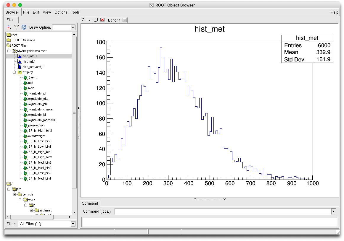
Since the option -n has been provided, the MyAnalysisName.root file does not only contain the defined histograms and regions, but also the ntuple variables:

root MyAnalysisName.root
(TFile *) 0x3396a90
root [1] .ls
TFile**         MyAnalysisName.root
 TFile*         MyAnalysisName.root
 KEY: TH1D     hist_met;1      hist_met
 KEY: TH2D     hist_metvsmt;1  hist_metvsmt
 KEY: TTree    ntuple;1        Simple Analysis ntuple

Investigating the ntuple tree, you can see that it not only contains the defined regions and variables, but also two branches called Event and eventWeight. While the Event branch containes event numbers (starting from 1) for each event, the eventWeight branch contains the MC event weight. In the region branches, each event that passed the region selection will be in 1, while the ones failing the region selection will be in 0.

Grid submission

Submission on the grid is rather straightforward

lsetup panda
mkdir $TUTORIAL_DIR/submit
cd $TUTORIAL_DIR/submit
ln -s $TUTORIAL_DIR/build/x86_64-centos7-gcc8-opt
prun --osMatching --exec 'source x86_64-centos7-gcc8-opt/setup.sh;simpleAnalysis -a ZeroLepton2015,ThreeBjets2015 %IN' --outputs='*.txt,*.root' --extFile \*.root --athenaTag 21.2.115,AnalysisBase --maxFileSize 40000000 --noCompile --followLinks --inDS <inputDS> --outDS user.<userName>.simple.v1

---

Last update: February 16, 2021